Chapter 3 Association–scatterplots

3.1 Basic elements of the grammar of graphics

TABLE 3.1: Summary of ggplot element.

ggplot element	Description
Data	ggplot uses a dataframe as input (e.g., data = mtcars.data)
Geoms	geometric element (e.g., geom_point, geom_bar)
Mapping	links data variables to aesthetic dimensions (aes) (e.g., aes(x = cyl, y = mpg))
Setting	specifies value of aesthetic dimension directly (e.g., colour = “blue”)
Layers	add components to base plot, most often geoms (additional layers added with “+”)
Stats	statistical summary, such as density or count; each geom has a default statistic
Position	adjusts the location of the plotted geom
Annotations	text and graphical overlays
Coordinate system	Cartesian, polar or small multiple facets
Themes	sets of plot parameters (e.g., font, background)

3.2 Simple scatterplot

The simplest plot must include data, aesthetic mapping, and geom a geometric element. The data must be organized with each observation as a row and each variable as a column. For a scatterplot the geometric element is a point, and the aesthetic mapping links variables to properties of the geometric element. For a scatterplot this would be the x and y position of the point. the the point the x and y position must be specified, but other properties, such as color, size, alpha level, and shape, can be mapped to variables. These properties of the geometric element can also be set to specific values, such as specifying the color of the point.

Figure ?? shows the ggplot2 code and associated scatterplot. The equation used to specify the plot implicitly specifies the values by their position, such as data being identifed as following “ggplot(”. The following speciifcations are equivalent:

library(tidyverse)

mtcars.df = mtcars

ggplot(data = mtcars.df, mapping = aes(x = wt, y = mpg)) +
  geom_point(colour = "darkblue")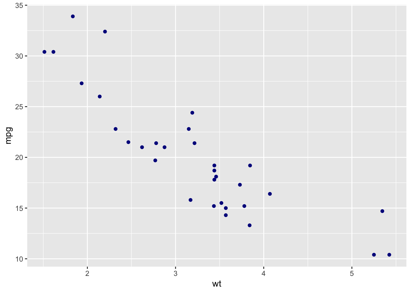

A powerful feature of ggplot2 is the abilty to add layers of geometric elements to a plot. Each layer can have its own data, mapping of aesthetic properties, and setting of aesthetic properties. The data and mapping specified in the base plot statement–“ggplot(data = mtcars.df, mapping = aes(x = wt, y = mpg))”–are global and apply to all layers, but can overridden by the any mappings specific to a layer.

Figure ?? shows a layer of red circles based on a subset of the data.

fourcyl.mtcars.df = mtcars.df %>% filter(cyl==4)

ggplot(data = mtcars.df, mapping = aes(x = wt, y = mpg)) +
  geom_point(colour = "darkblue") + 
  geom_point(data = fourcyl.mtcars.df, colour = "red", shape = 21, size = 4)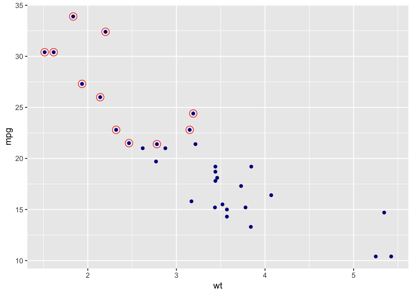

3.3 Scatterplot with additional mappings

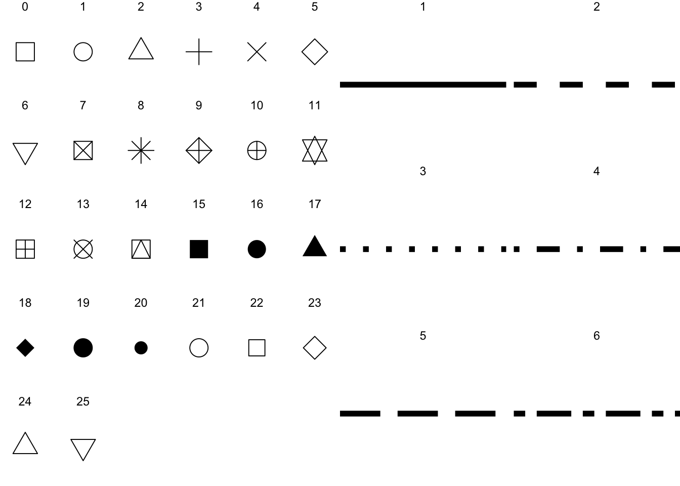
The scatterplot typically maps variables to the x and y position of the points, but ggplot allows for other mappings. Figure ?? shows mapping variables to the fill and size of the points. The shape, stroke, and color of the points are set to values they could also be mapped, which could quickly overload the graph. Note that only shapes 21-25 in Figure ?? can include fill and stroke, with the other symbols color determines the color of the whole symbol not just the border.

ggplot(data = mtcars, mapping = aes(x = wt, y = mpg, fill = hp, size = 1/qsec)) + 
  geom_point(shape = 21, colour = "darkred", stroke = 2.)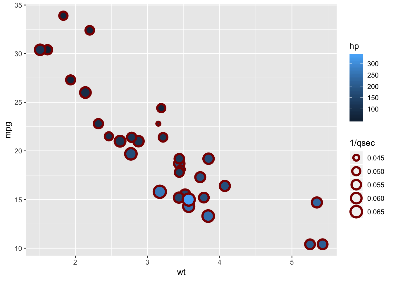 

library(RColorBrewer)

display.brewer.all(type="qual")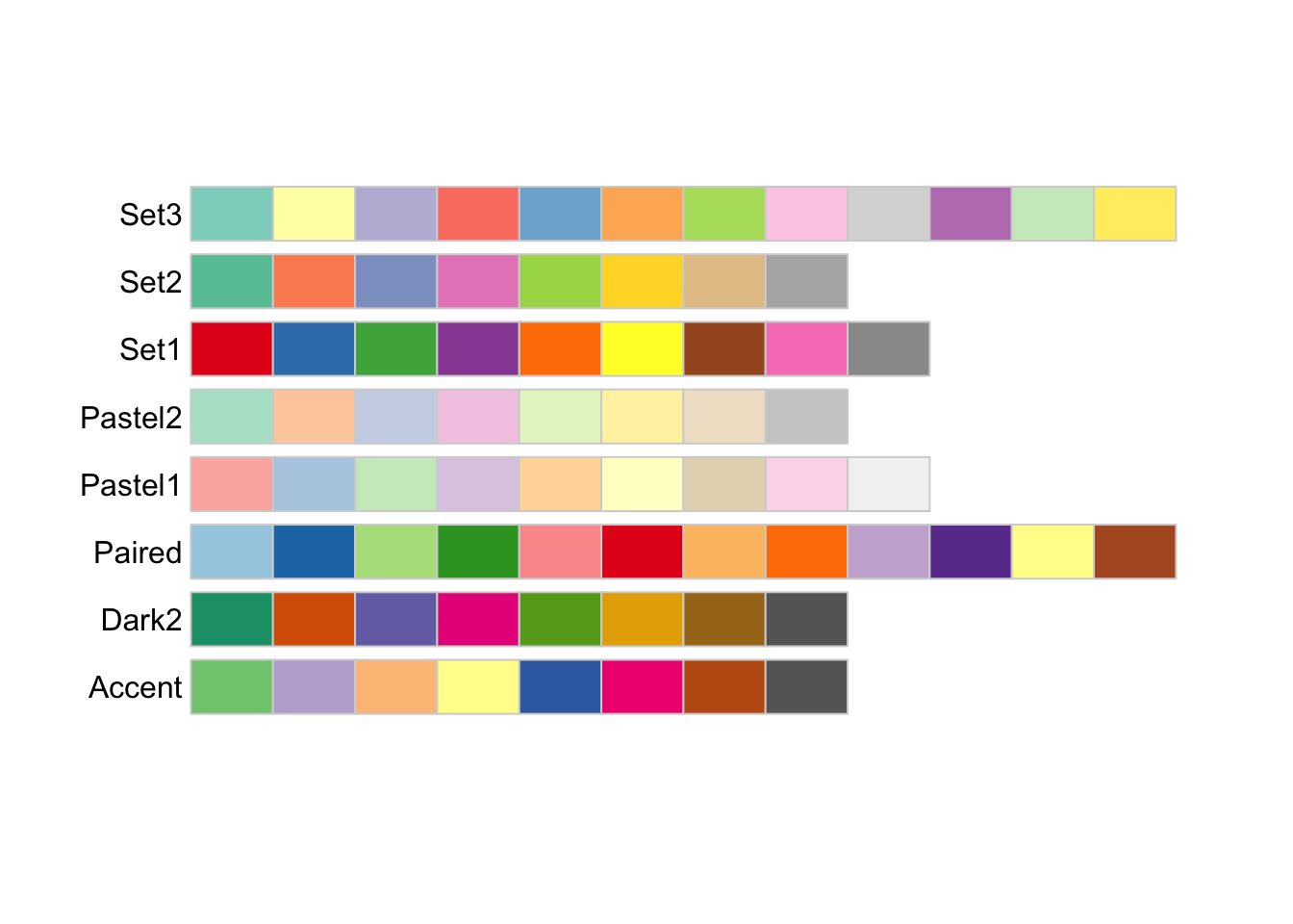

display.brewer.all(type="seq")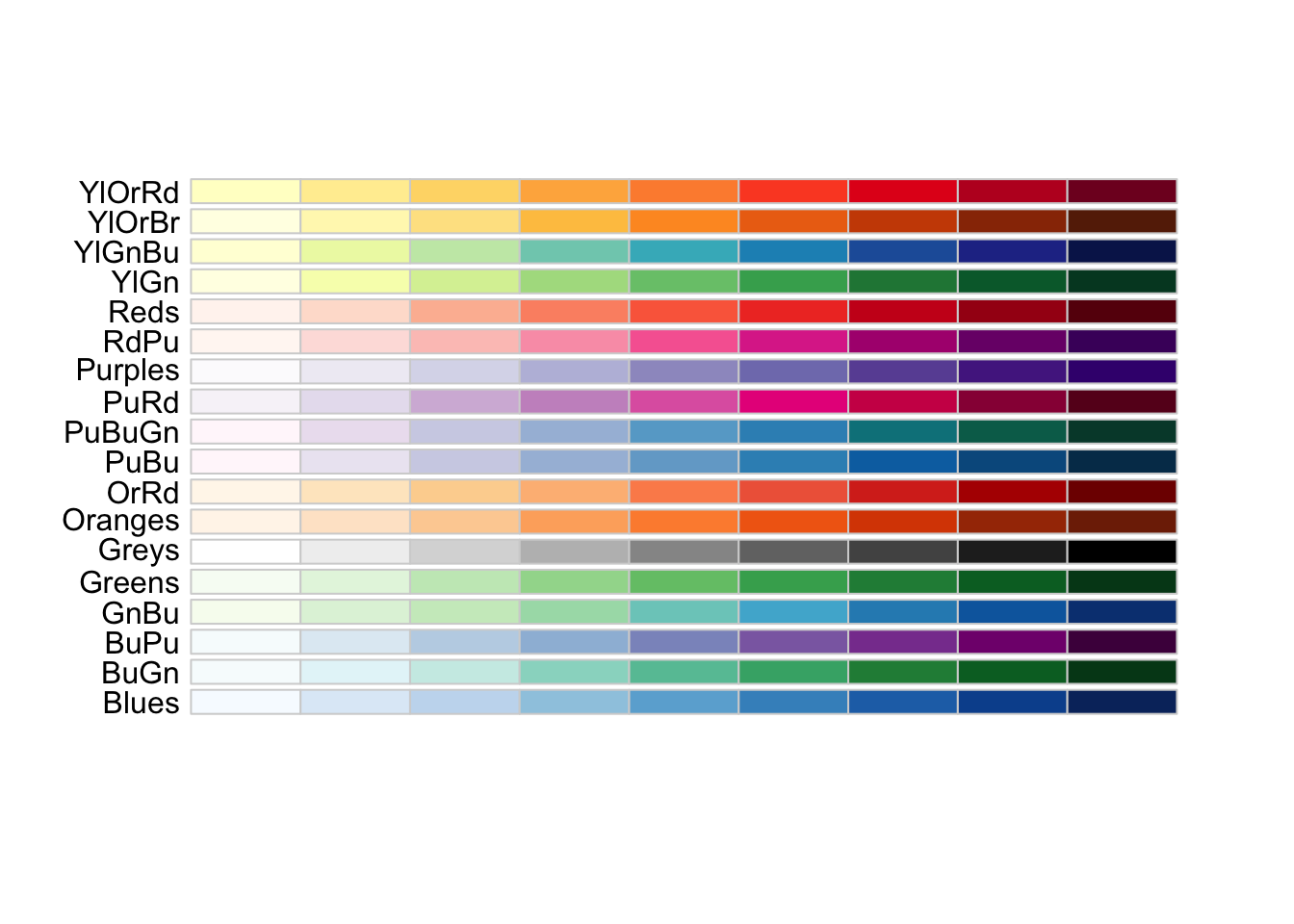

display.brewer.all(type="div")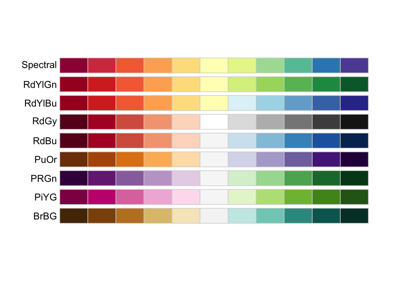

# display.brewer.all(n=NULL, type="all", 
#                    select=NULL, exact.n=TRUE, 
#                    colorblindFriendly=FALSE)

3.4 Scatterplot with linear and loess fit

The layers can include geometric elements beyond geom_point. Perhapts the most useful geoms to add to a scatterplot is a curve fit. Figure ?? shows a simple scatterplot with two cruve fits. The loess fit shows a smooth fit that indicates non-linar trends, and the blue line shows a linear regeression. The loess line highligths areas in the data that deviate from a linear relationship shown by the blue line. All three layers inherit the same x and y mapping from the ggplot base layer.

When building a plot each layer is placed on top of the preceding layer, such that the last layer lies on top of all the others. With Figure ??, the points are on the bottom and the light blue line is on top of the gray loess line.

Table ?? shows the full set of possible geometric elements that can be used to create graphs, the following chapters describe many of these.

Note the smooth fit geoms include additional settings for the method and whether the line should include a standard error.

ggplot(data = mtcars.df, aes(x = wt, y = mpg)) +
  geom_point(colour = "darkblue") +
  geom_smooth(method = "loess", se = FALSE, colour = "darkgrey") + 
  geom_smooth(method = "lm", fill = "lightblue")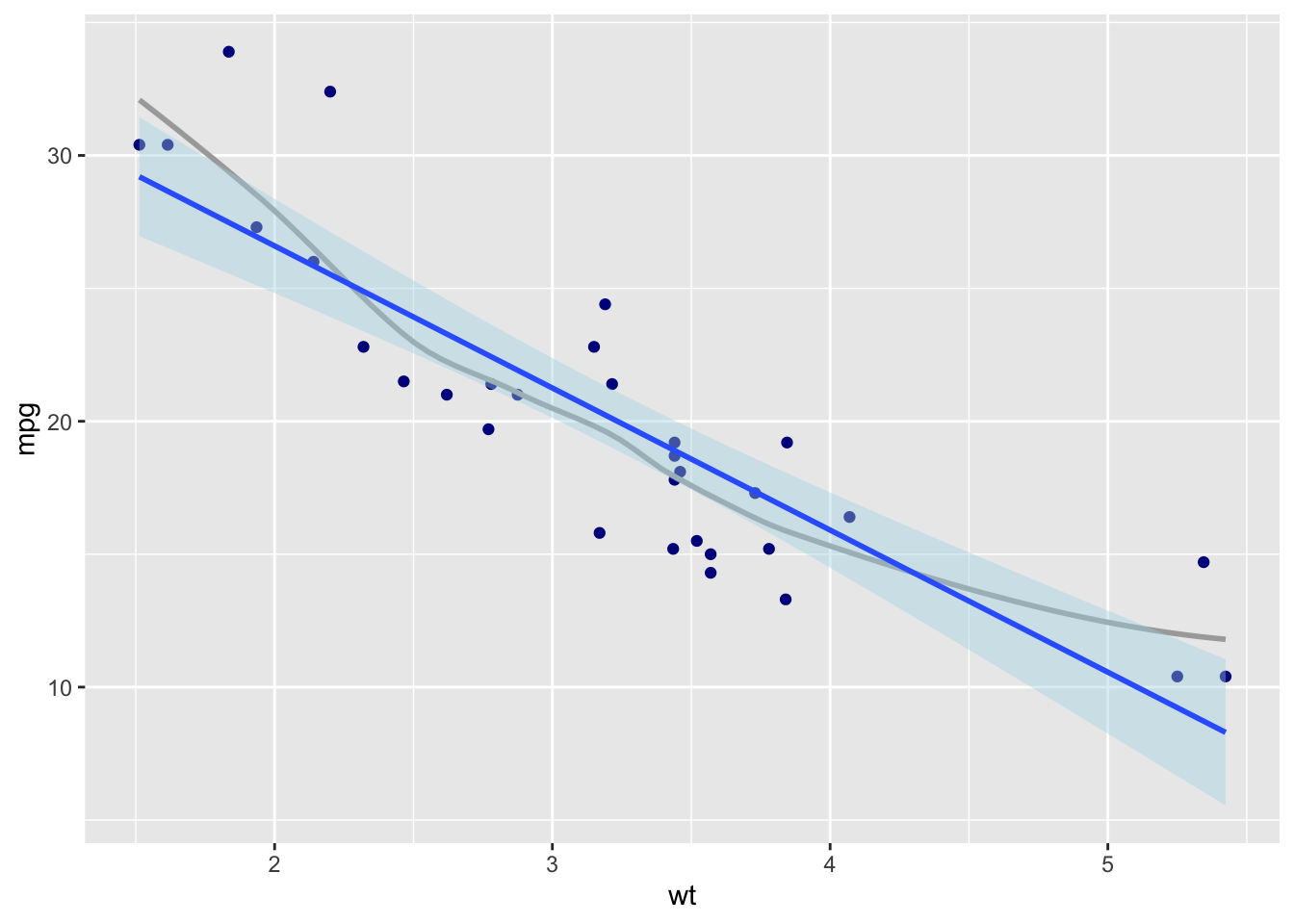

x
geom_abline
geom_area
geom_bar
geom_bin2d
geom_blank
geom_boxplot
geom_col
geom_contour
geom_count
geom_crossbar
geom_curve
geom_density
geom_density_2d
geom_density2d
geom_dotplot
geom_errorbar
geom_errorbarh
geom_freqpoly
geom_hex
geom_histogram
geom_hline
geom_jitter
geom_label
geom_line
geom_linerange
geom_map
geom_path
geom_point
geom_pointrange
geom_polygon
geom_qq
geom_qq_line
geom_quantile
geom_raster
geom_rect
geom_ribbon
geom_rug
geom_segment
geom_sf
geom_sf_label
geom_sf_text
geom_smooth
geom_spoke
geom_step
geom_text
geom_tile
geom_violin
geom_vline

3.5 Global and local regression

ggplot(data = mtcars.df, aes(x = wt, y = mpg)) +
  geom_smooth(method = lm, colour = "darkgrey", size = .5) +
  geom_point(aes(colour = as.factor(cyl))) +
  geom_smooth(aes(colour = as.factor(cyl)), method = lm, se = FALSE)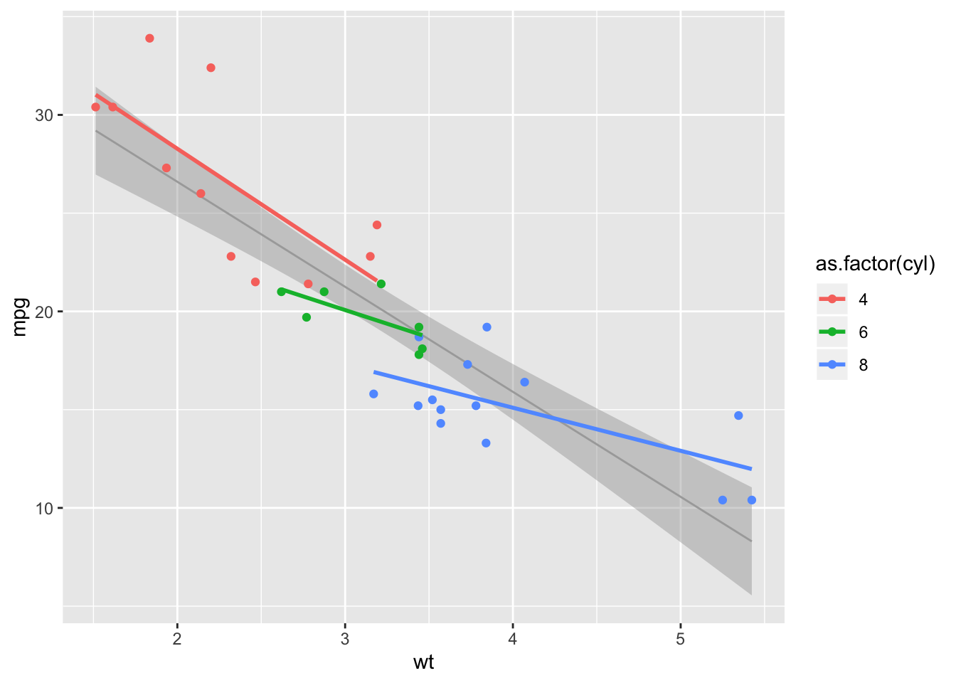

3.6 Quantile regression and other functional relationships

Often the question the graph is meant to answer is not about the central tendency, but about the likelihood of relatively extreme values, such as the 25th and 75th percentiles.

ggplot(data = mtcars.df, aes(x = wt, y = mpg)) +
    geom_smooth(method = lm, colour = "darkgrey", size = .5) +
  geom_point() +
  geom_quantile(quantiles = c(.25, .75))

## Smoothing formula not specified. Using: y ~ x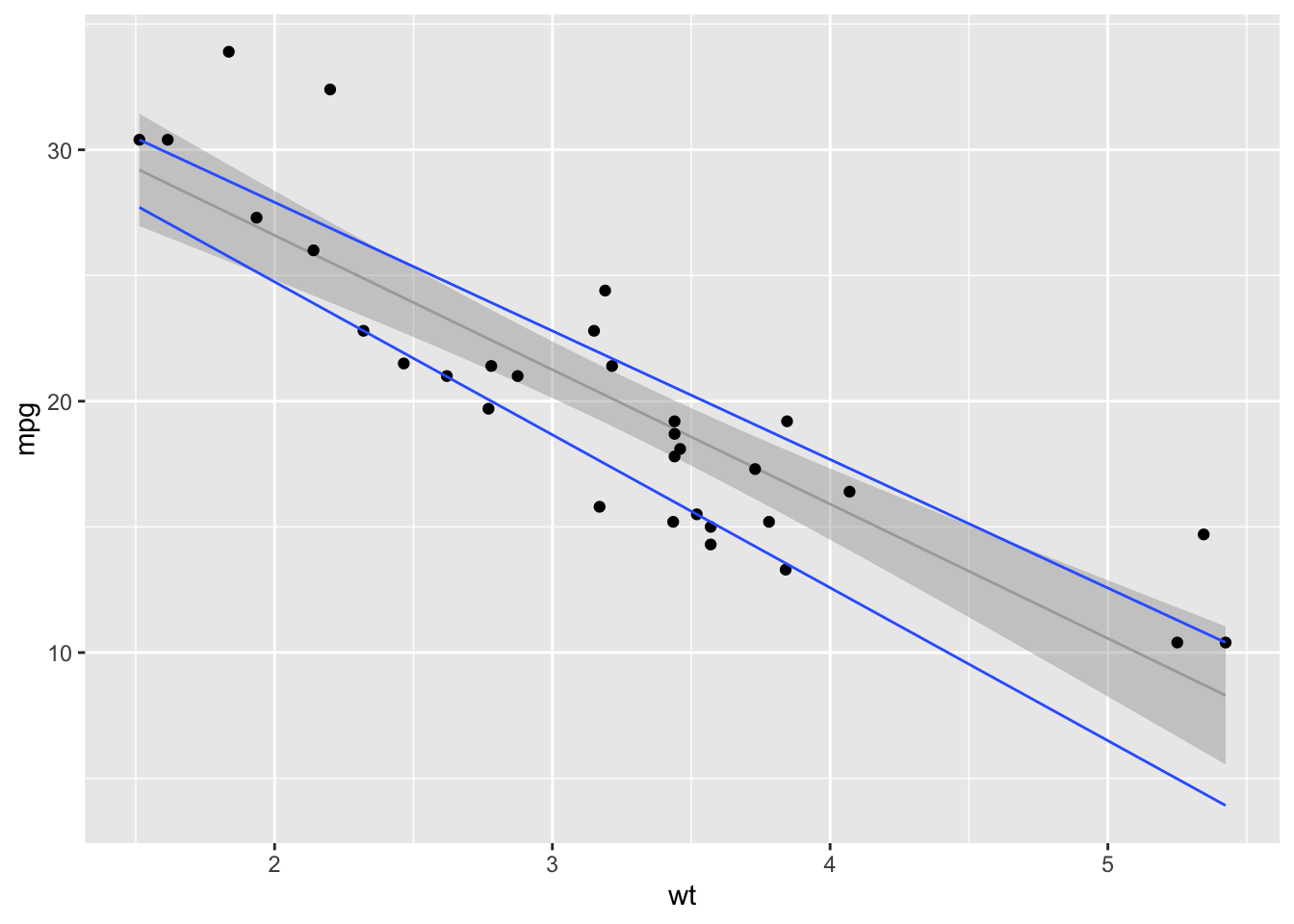

3.7 Scatterplot with regression equation and marginal distributions

Scatterplot augmented with marginal distributions, regression equation, and Tufte-inspired range frame.

Marginal distributions show that a 1-D scatterplot is a histogram and that a 2-d histogram is a scatterplot. Chapter 4 describes such plots in detail.

Chapter 10 shows how to add annotations, such as the equation.

Derived from: http://t-redactyl.io/blog/2016/05/creating-plots-in-r-using-ggplot2-part-11-linear-regression-plots.html

library(ggthemes)
library(ggExtra) # For marginal histograms

mtcars.df = mtcars

equation = function(x) {
  lm_coef <- list(a = round(coef(x)[1], digits = 2),
                  b = round(coef(x)[2], digits = 2),
                  r2 = round(summary(x)$r.squared, digits = 2));
  lm_eq <- substitute(italic(y) == a + b %.% italic(x)*","~~italic(R)^2~"="~r2,lm_coef)
  as.character(as.expression(lm_eq));                 
}


fit = lm(mpg~wt, data = mtcars.df)

p = ggplot(mtcars.df, aes(x=wt, y=mpg)) + 
  geom_point(colour = "darkblue") + 
  geom_smooth(method=lm, se=FALSE) +
  annotate("text", x = 4, y = 30, label = equation(fit), parse = TRUE) +
  geom_rangeframe() + # Requires ggthemes 
  theme_minimal()

p = ggMarginal(p, type = "histogram")
p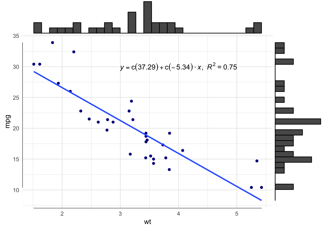

3.8 Categorical scatterplot

mtcars.df = mtcars
mtcars.df$gear = as.factor(mtcars.df$gear)
mtcars.df$am = as.factor(mtcars.df$am)

ggplot(mtcars.df, aes(gear, am)) + 
  geom_count()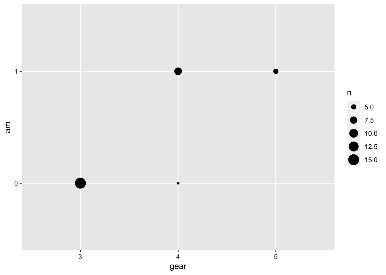

 ggplot(mtcars.df, aes(gear, am)) + 
  geom_jitter(width = 0.075, height = 0.075)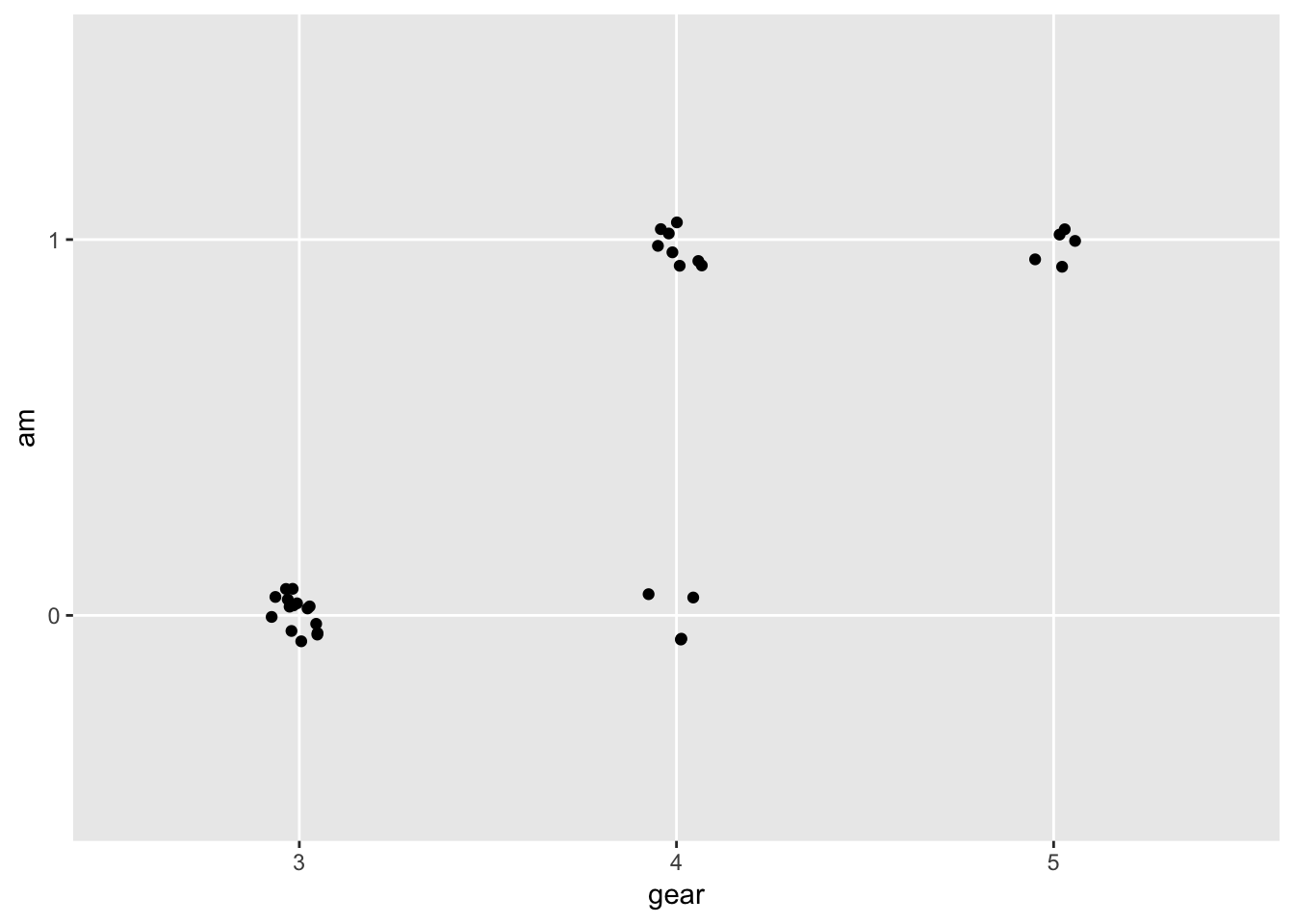 

s.mtcars.df = mtcars.df %>% group_by(gear, am) %>% summarise(count = n())

ggplot(s.mtcars.df, aes(gear, am)) + 
  geom_tile(aes(fill = count))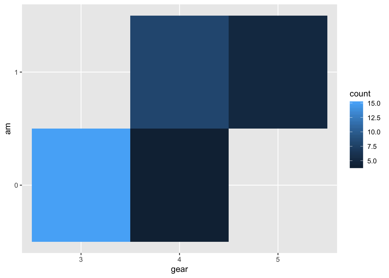

3.9 Table lens

Table lens serves a similar purpose to the scatterplot but might be more familiar and focusses attention on individual variables and individual cases. Chapter 9 provides more detail on this technique.

3.10 Scatterplot with overplotting mitigation

diamonds.df = diamonds

ggplot(diamonds.df, aes(carat, price)) +
  geom_point()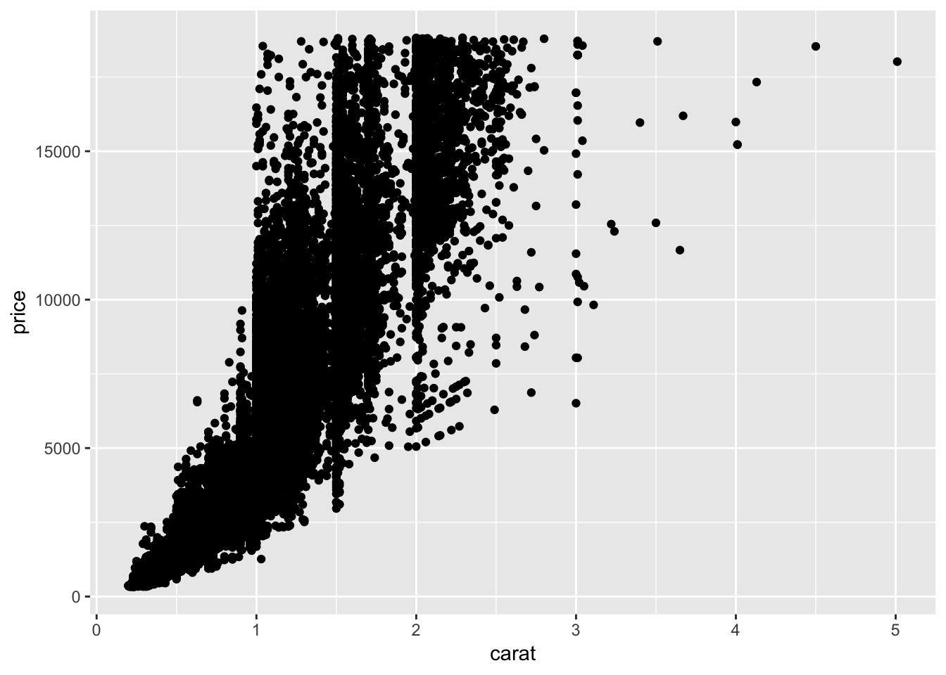

ggplot(diamonds.df, aes(carat, price)) +
  geom_point(size = .1)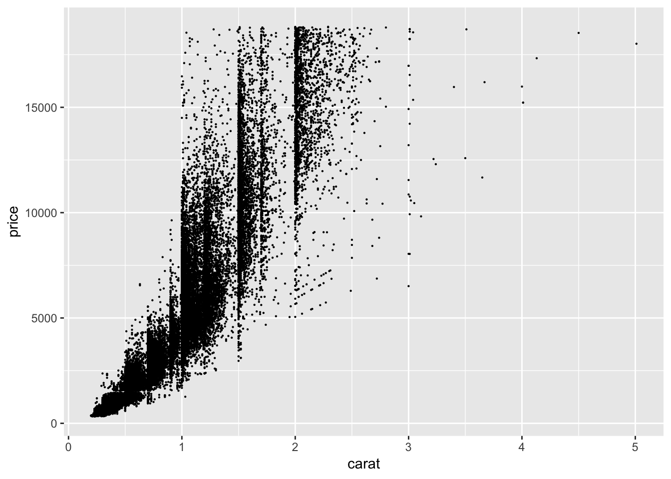

ggplot(diamonds.df, aes(carat, price)) +
  geom_point(size = .3, shape = 21)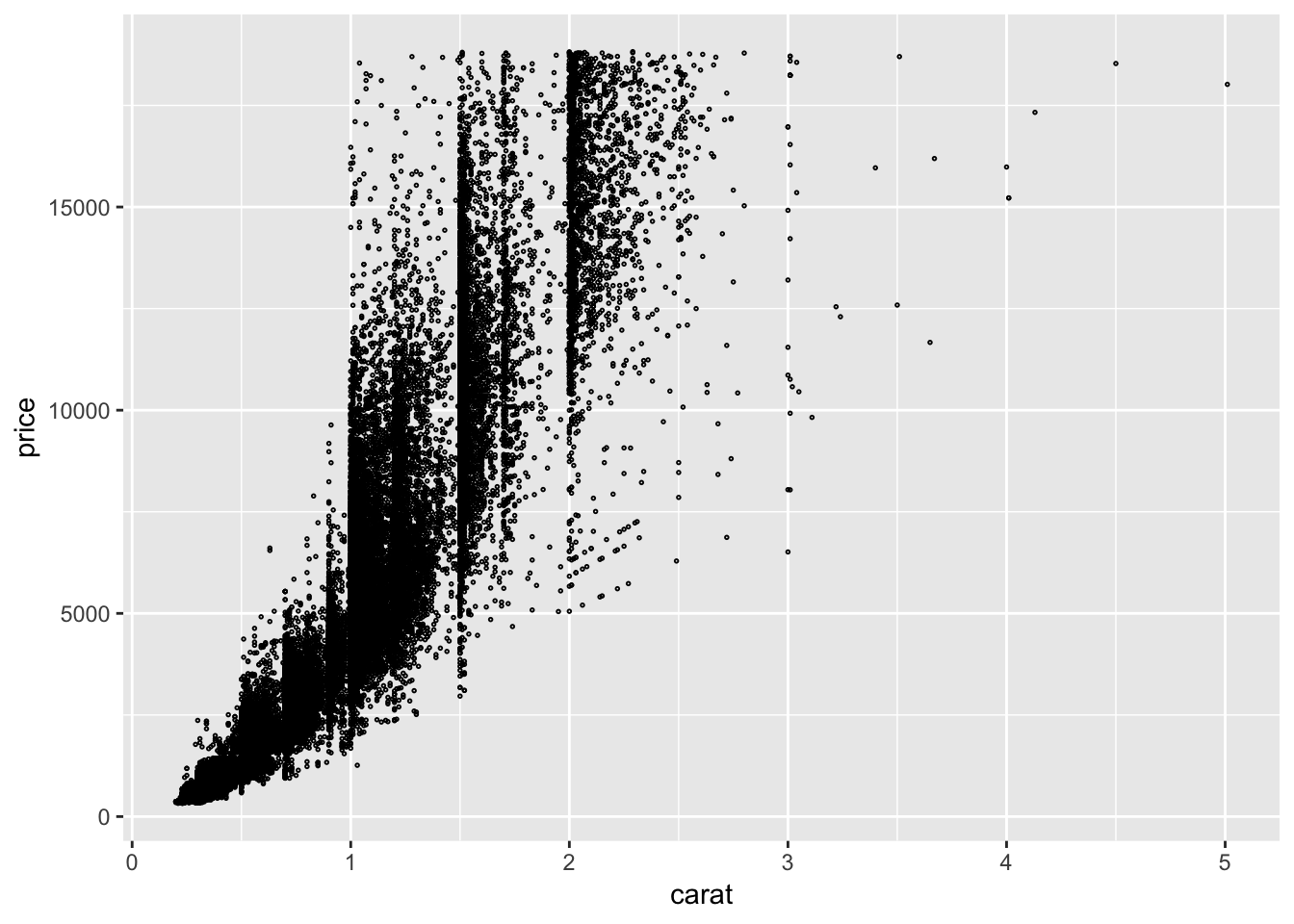

ggplot(diamonds.df, aes(carat, price)) +
  geom_point(size = .3, shape = 21, alpha = .3)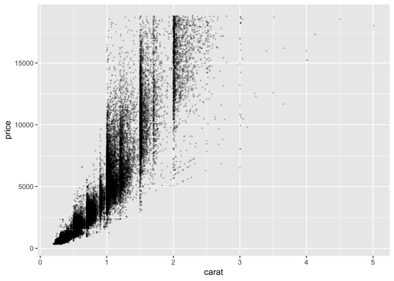

ggplot(diamonds.df %>% sample_n(10000), aes(carat, price)) +
  geom_point(size = .3, shape = 21, alpha = .3)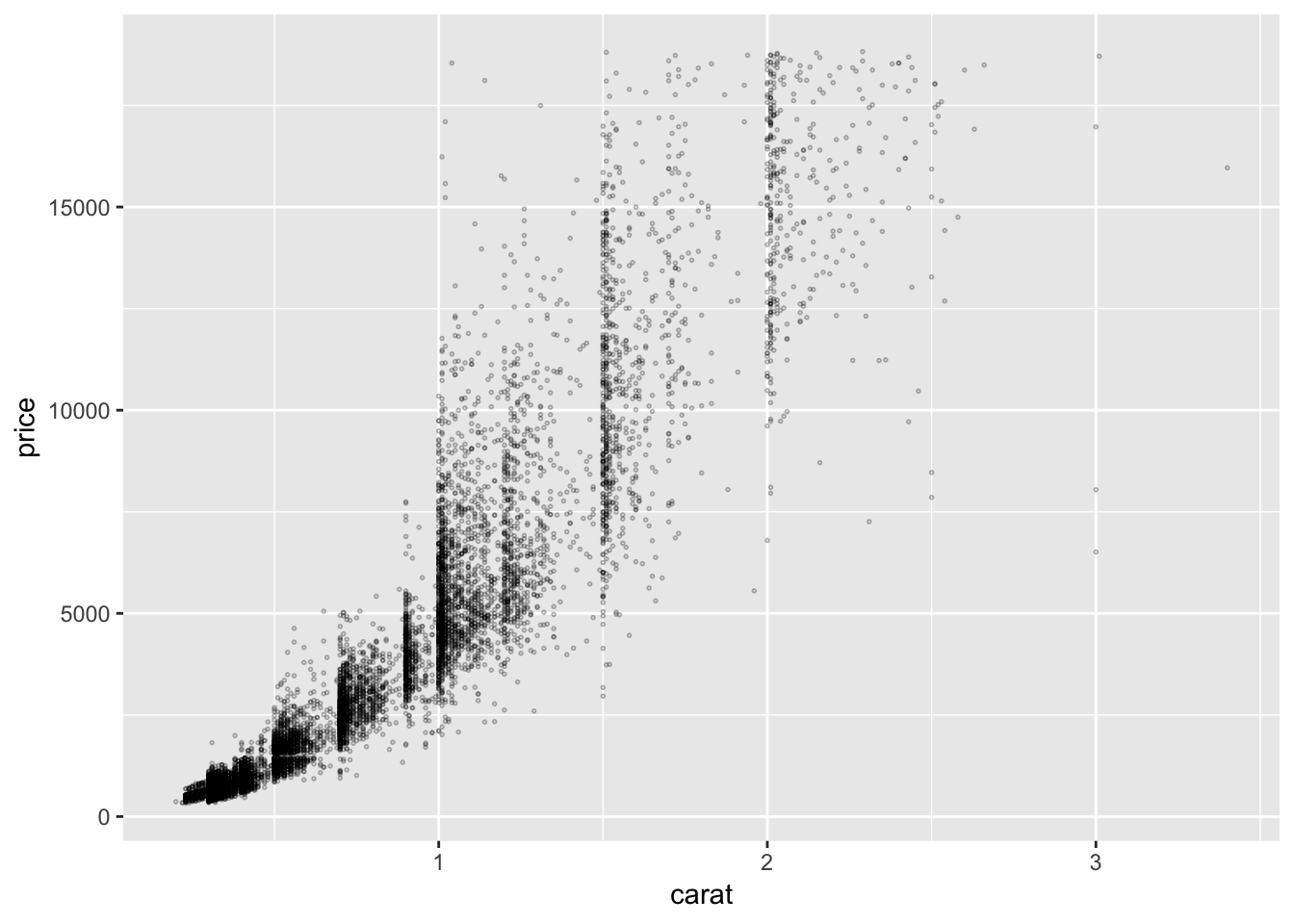

ggplot(diamonds.df, aes(log(carat), log(price))) +
  geom_point(size = .3, shape = 21, alpha = .3)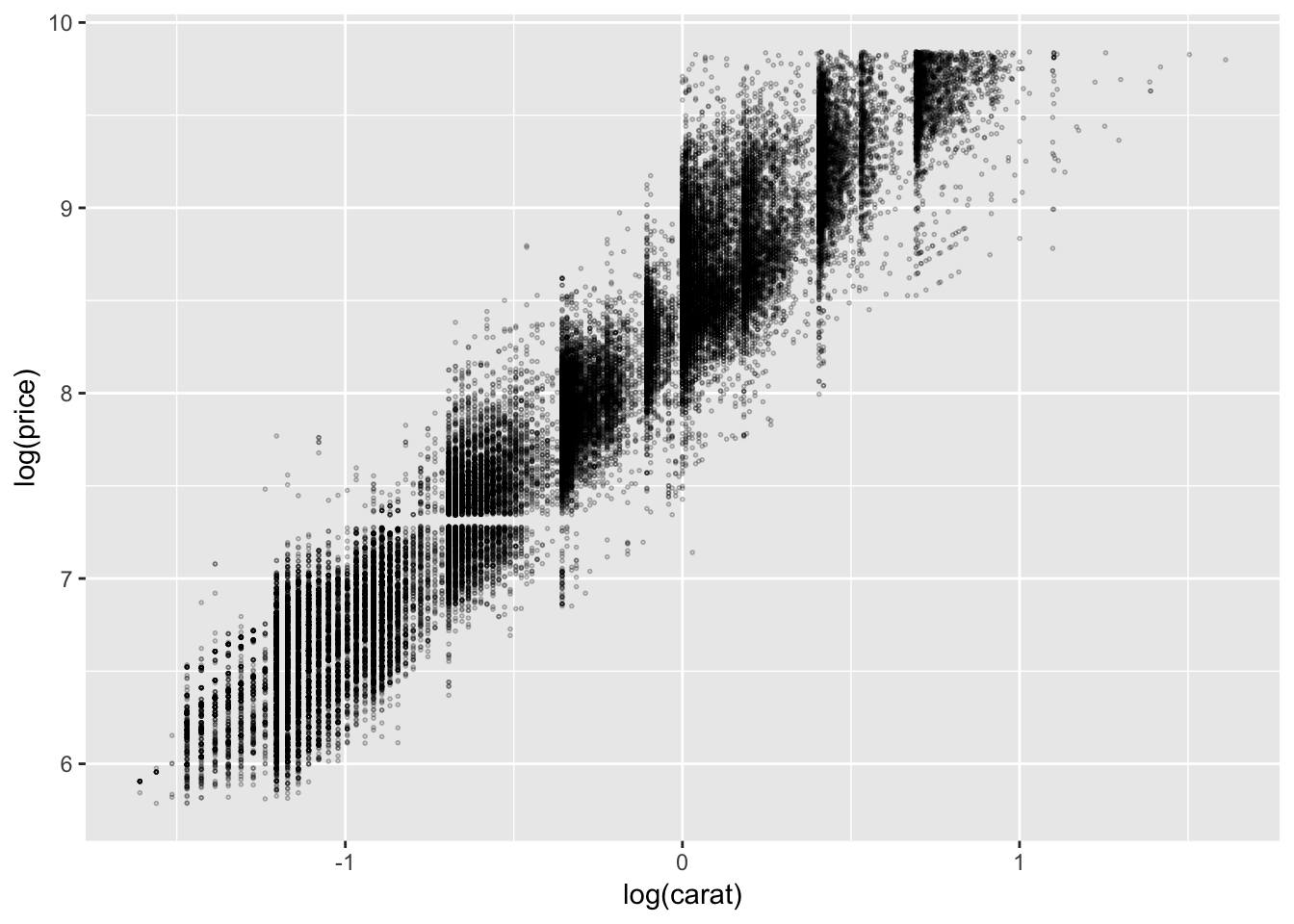

ggplot(diamonds.df, aes(log(carat), log(price))) +
  geom_count(show.legend=F, alpha =.3, shape =21)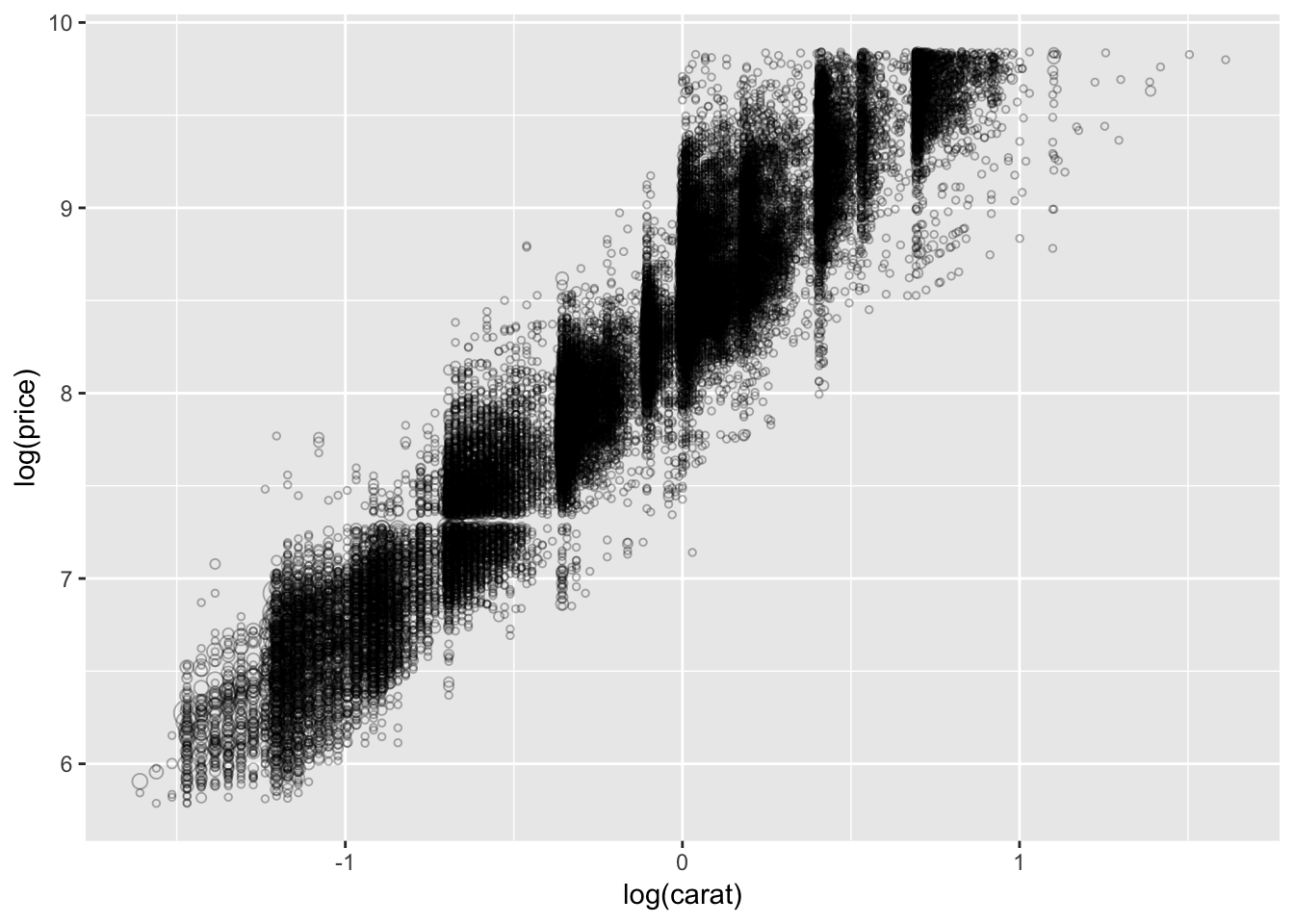

ggplot(data = mtcars.df, aes( x = disp, y = hp)) +
  geom_point(colour = "grey40", shape = 21)+
  geom_smooth(method = loess, colour = "grey40")+
  geom_smooth(method = lm, se = FALSE, size = .75) +
    geom_smooth(aes(colour = factor(cyl)), 
        method = lm, se = FALSE, size = 1.5)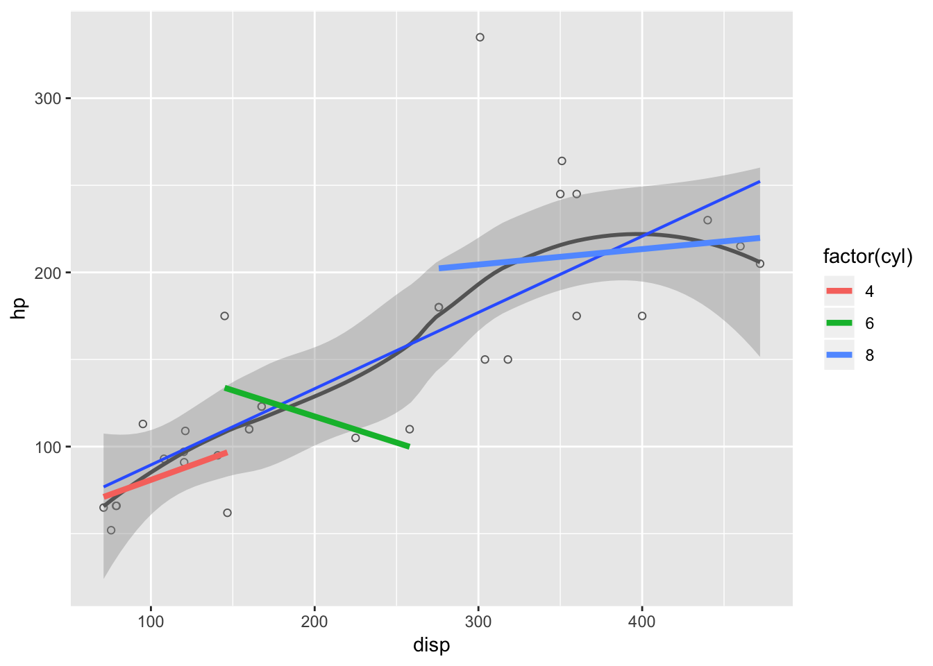

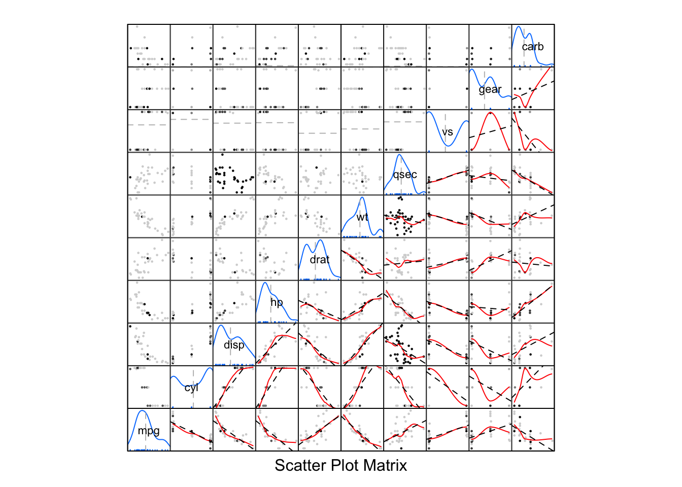
3.11 A matrix of scatterplots

##  [1] "mpg"  "cyl"  "disp" "hp"   "drat" "wt"   "qsec"
##  [8] "vs"   "am"   "gear" "carb"