Chapter 4 Distribution–histograms and density plots

library(tidyverse)
library(HistData)
library(ggpubr)

4.1 Histograms and bin choice

Seeing the smooth and rough of data bins or binwidth, default number of bins is 30

h10.plot = ggplot(data = diamonds.df, aes(price)) + 
  geom_histogram(bins = 10) 

h30.plot = ggplot(data = diamonds.df, aes(price)) + 
  geom_histogram(bins = 30) 

h80.plot = ggplot(data = diamonds.df, aes(price)) + 
  geom_histogram(bins = 80) 

ggarrange(h10.plot, h30.plot, h80.plot,
    nrow=1, ncol = 3, align = "h")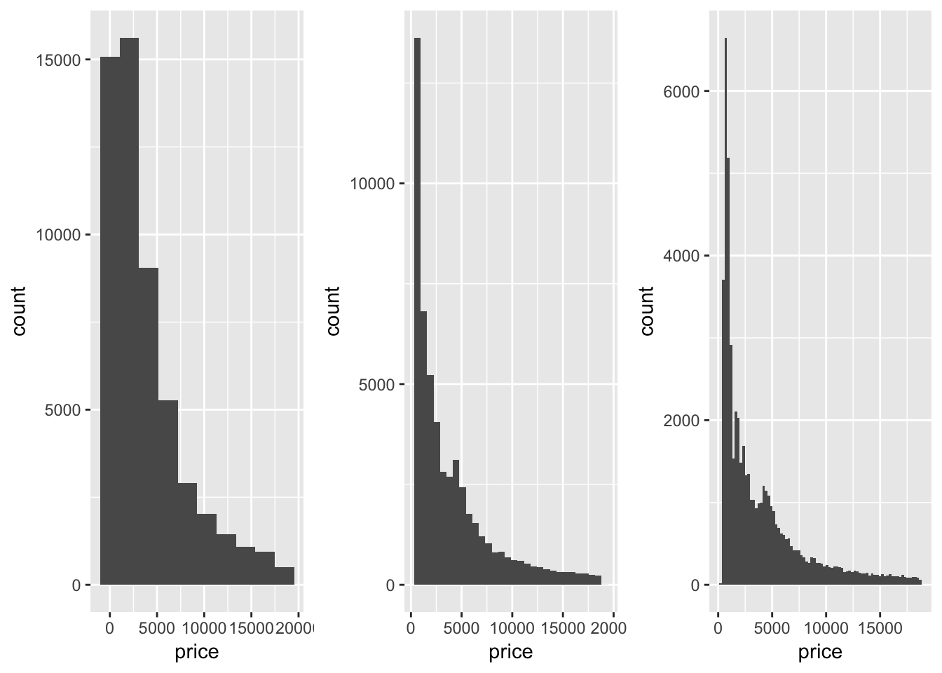

4.2 Density and kernel adjustment

Density as abstraction and model

Adjust is a multiplier on the default kernel bandwidth and so 1 represents the default

a10.plot = ggplot(data = diamonds.df, aes(price)) + 
  geom_density(adjust = 10) 

a1.plot = ggplot(data = diamonds.df, aes(price)) + 
  geom_density(adjust = 1) 

a01.plot = ggplot(data = diamonds.df, aes(price)) + 
  geom_density(adjust  = 0.1) 

ggarrange(a10.plot, a1.plot, a01.plot,
    nrow=1, ncol = 3, align = "h")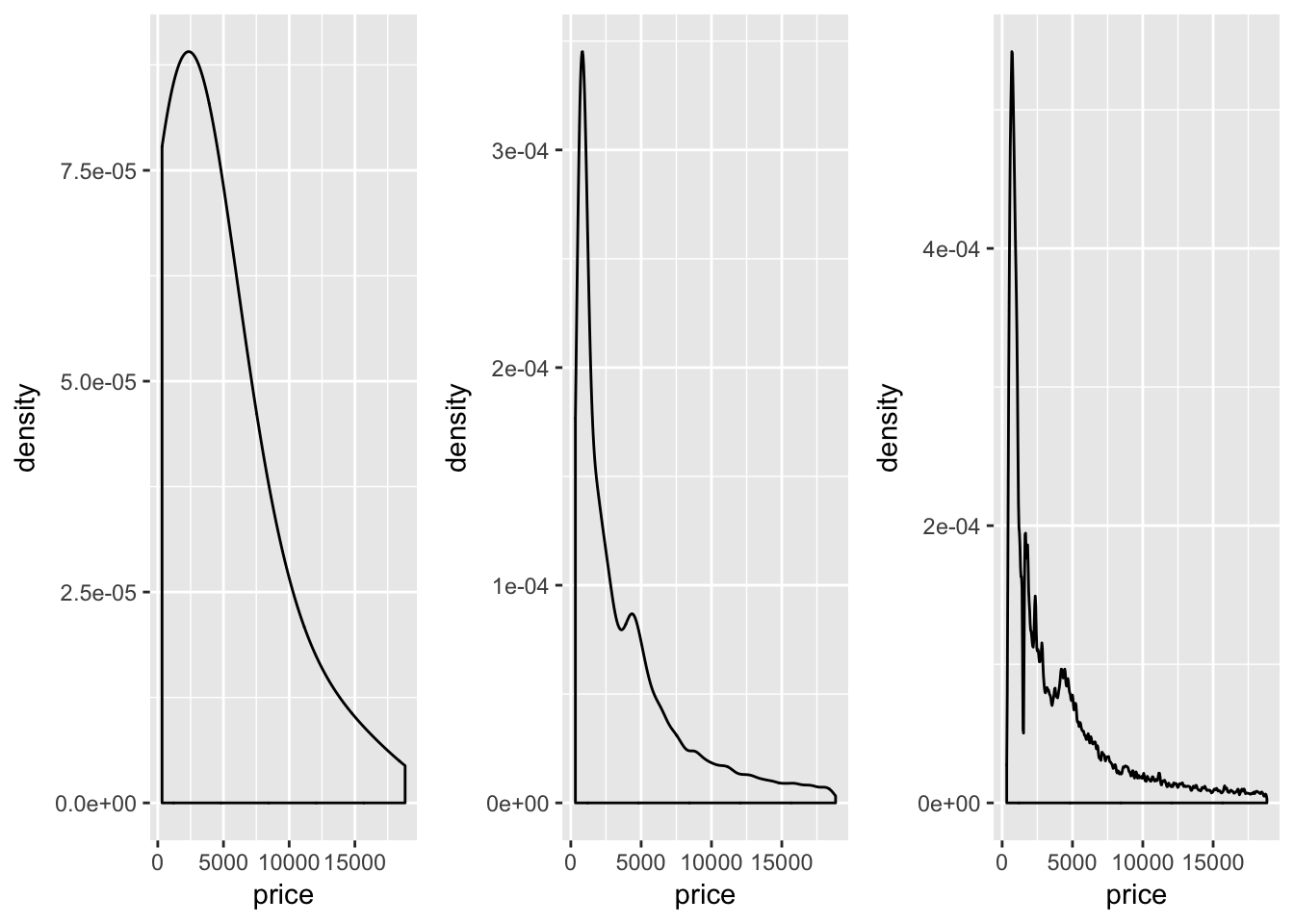

4.3 Histogram percentage rather than count

library(scales)

ggplot(mtcars.df , aes(x = as.factor(cyl))) + 
    geom_bar(aes(y = (..count..)/sum(..count..))) + 
    scale_y_continuous(labels = scales::percent)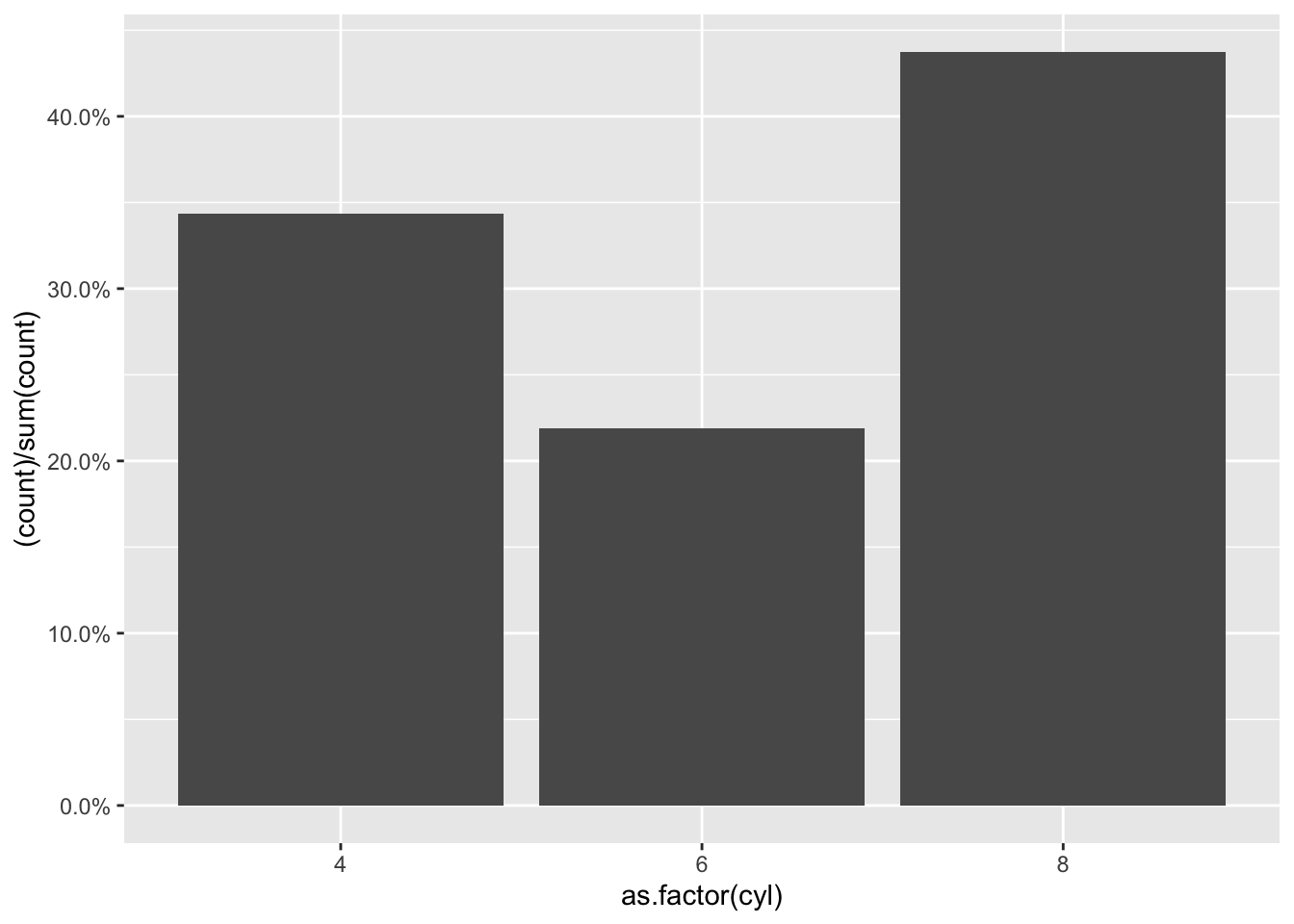

4.4 Histogram, density overlay, and normal overlay

4.5 Cummulative density

diamonds.df = diamonds

ggplot(diamonds.df, aes(price, colour = cut)) + 
  stat_ecdf(geom = "step")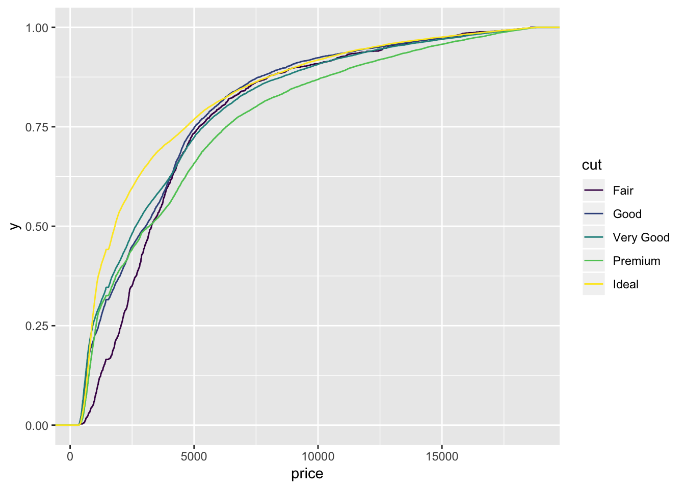

4.6 Quantile-quantle plot

Plots quantiles of sample as a function of the quantiles of the theoretical distribution.

ggplot(diamonds.df, aes(sample = price)) + 
  geom_qq(distribution = qlnorm) +
  geom_abline(intercept = mean(diamonds.df$price), slope = sd(diamonds.df$price))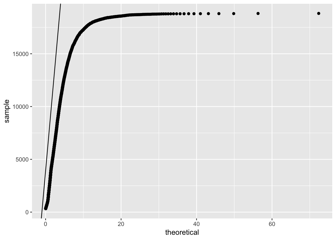

4.7 Cummulative density

ggplot(diamonds.df, aes(price, colour = cut)) + 
  stat_ecdf(geom = "step")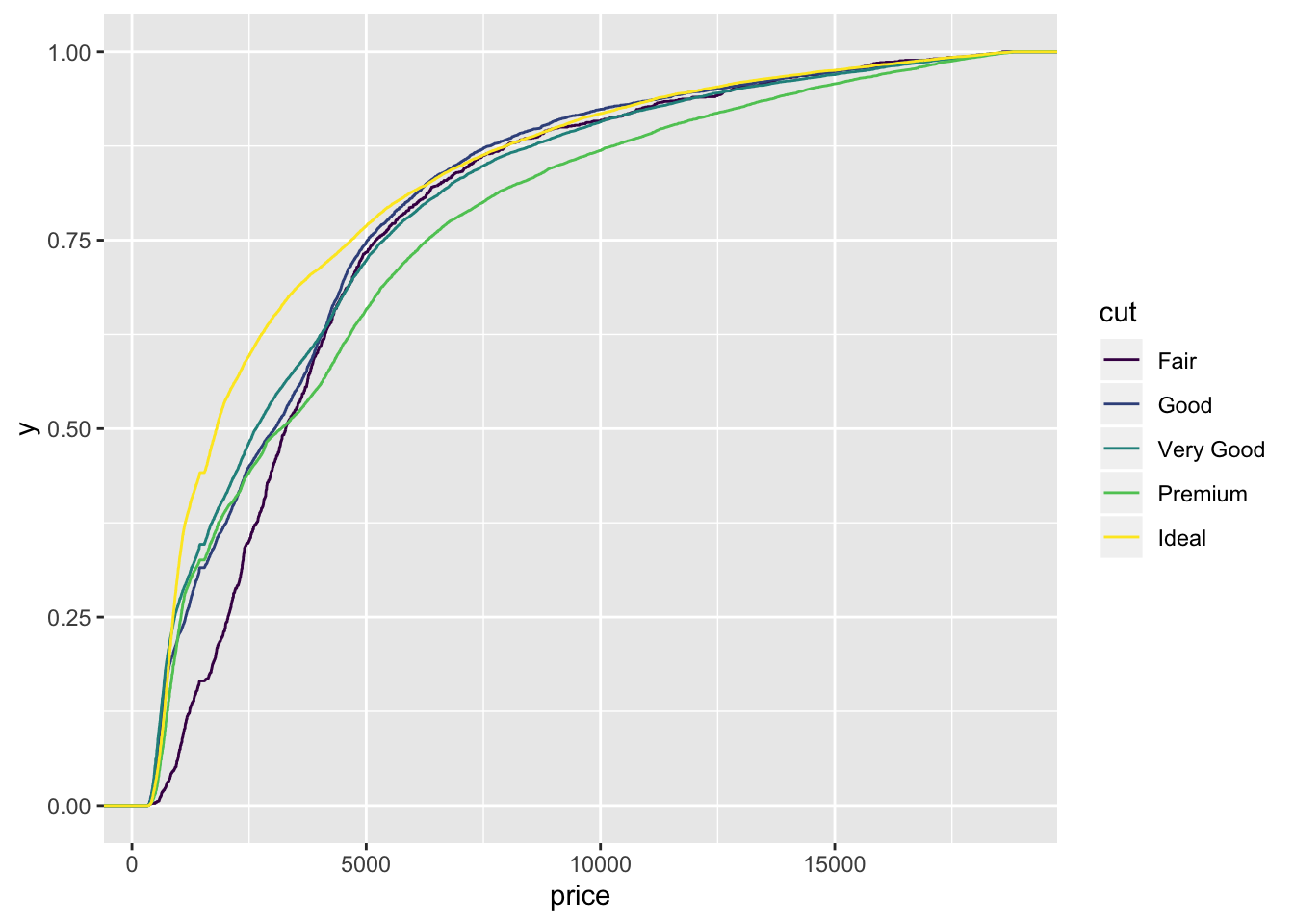

4.8 Distribution: 2-D distribution and overplotting revisited

ggplot(diamonds.df, aes(log(carat), log(price)))+
  geom_point(alpha = .01)+ 
  theme_bw()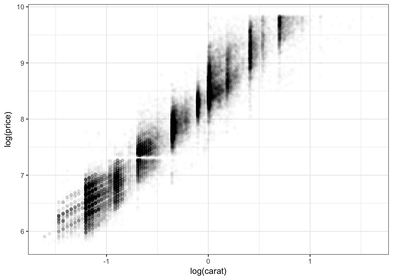

ggplot(diamonds.df, aes(log(carat), log(price)))+
  geom_point(size = .5)+ 
  geom_density2d(size=1.2)+
  theme_bw()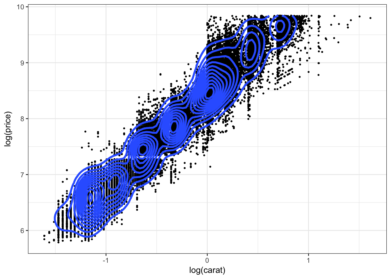

ggplot(diamonds.df, aes(log(carat), log(price)))+
  geom_point(size = .5)+ 
  geom_density2d(size=1.2)+
  geom_hex(alpha = .6) +
  theme_bw()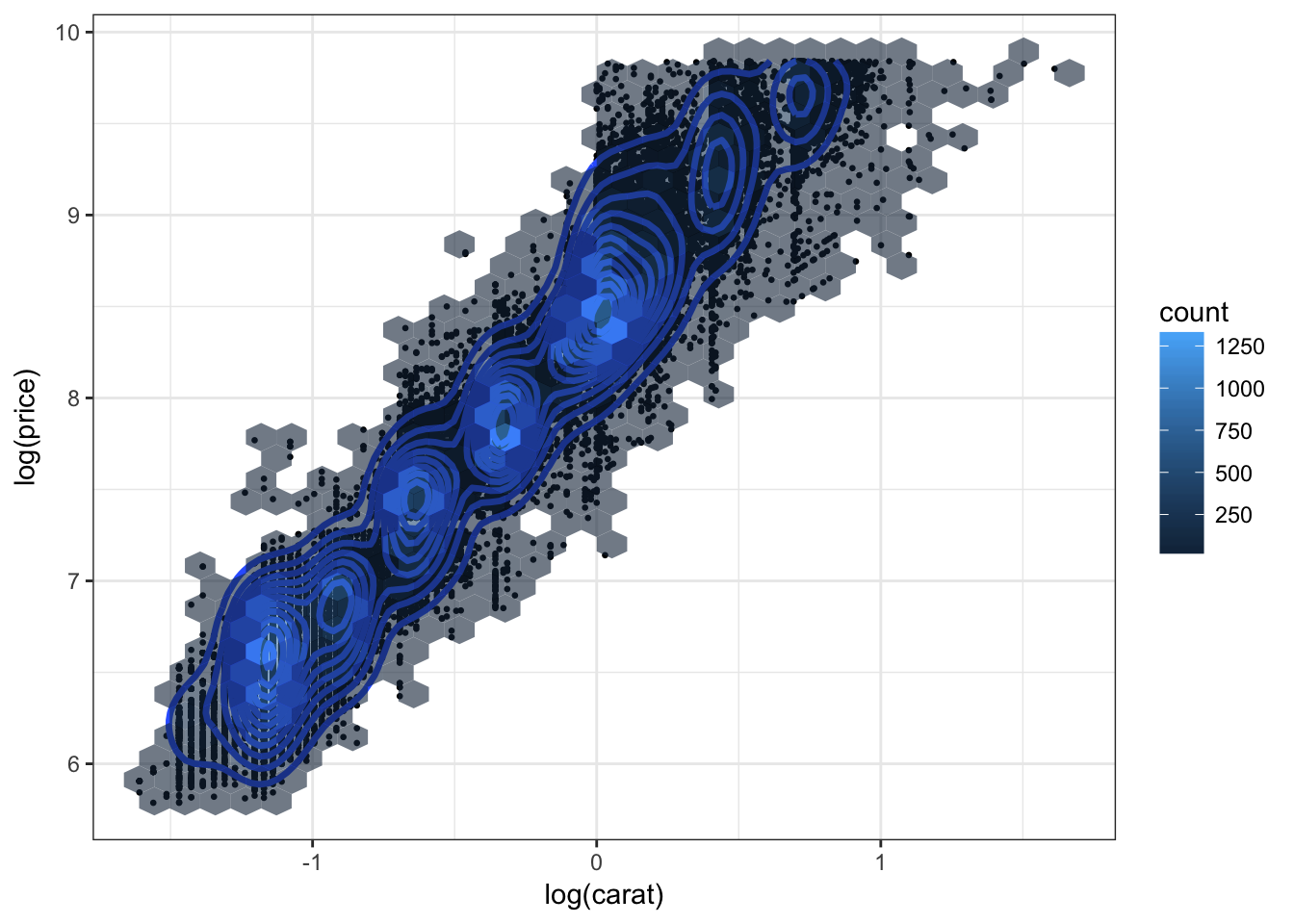

ggplot(diamonds.df, aes(log(carat), log(price)))+
  #geom_point( )+
  #geom_point(size = .5)+ 
  #geom_density2d(size=1.2)+
  geom_hex(bins = 50) +
  theme_bw()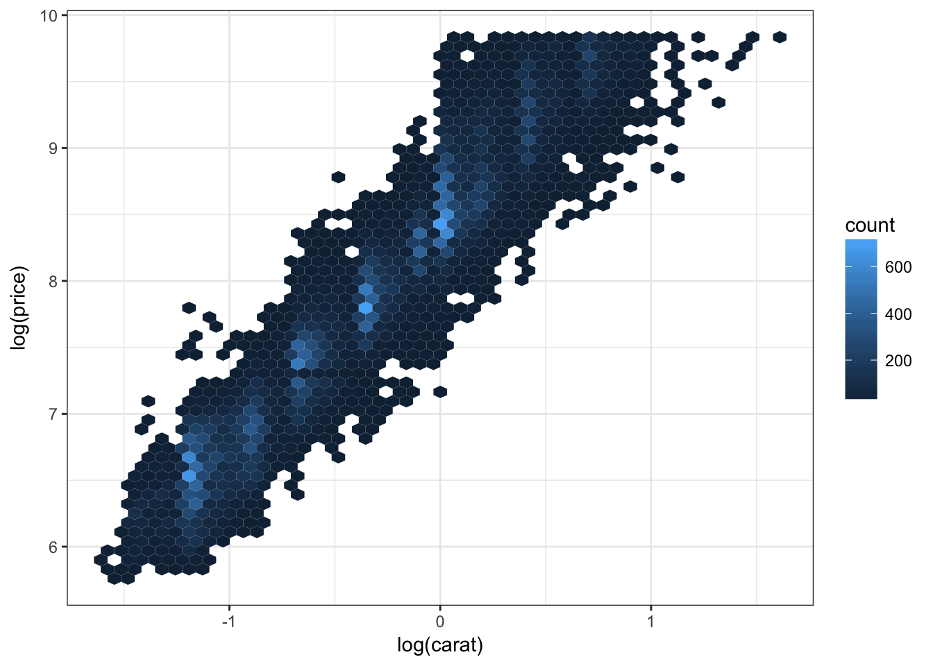

4.9 Small multiple histogram with density and median reference lines

TODO change to diversity data gender across job types

diamonds.df = diamonds

sum.diamonds.df = diamonds.df %>% group_by(cut) %>% 
  summarise(q85 = quantile(price, 0.85))

ggplot(data = diamonds.df, aes(price)) + 
  geom_histogram(aes(y = ..density..), bins = 40) + 
  geom_density(colour = "darkblue") +
  geom_vline(data = sum.diamonds.df, aes(xintercept = q85)) +
  facet_grid(cut ~ .)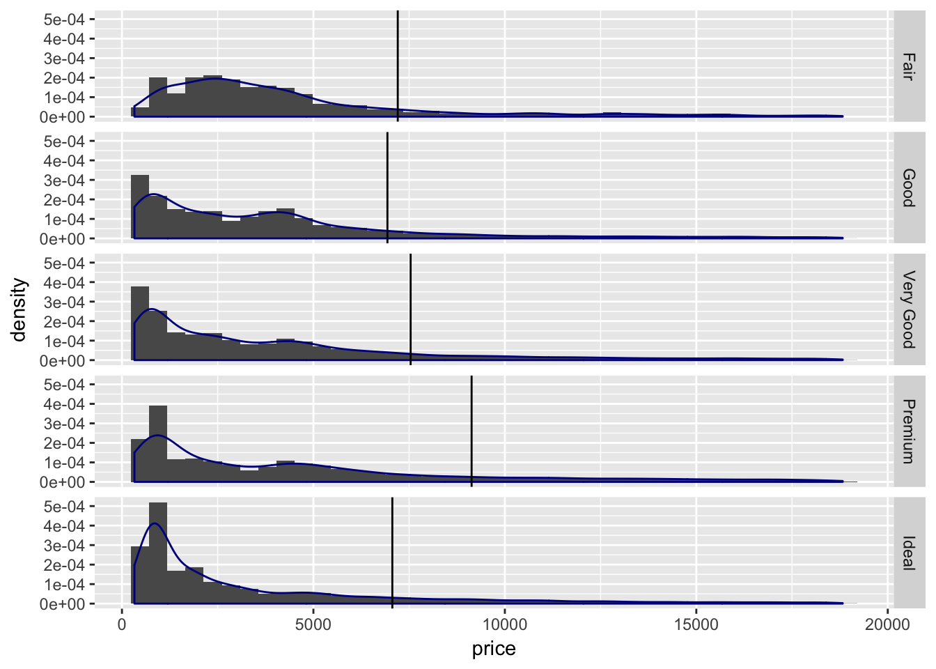

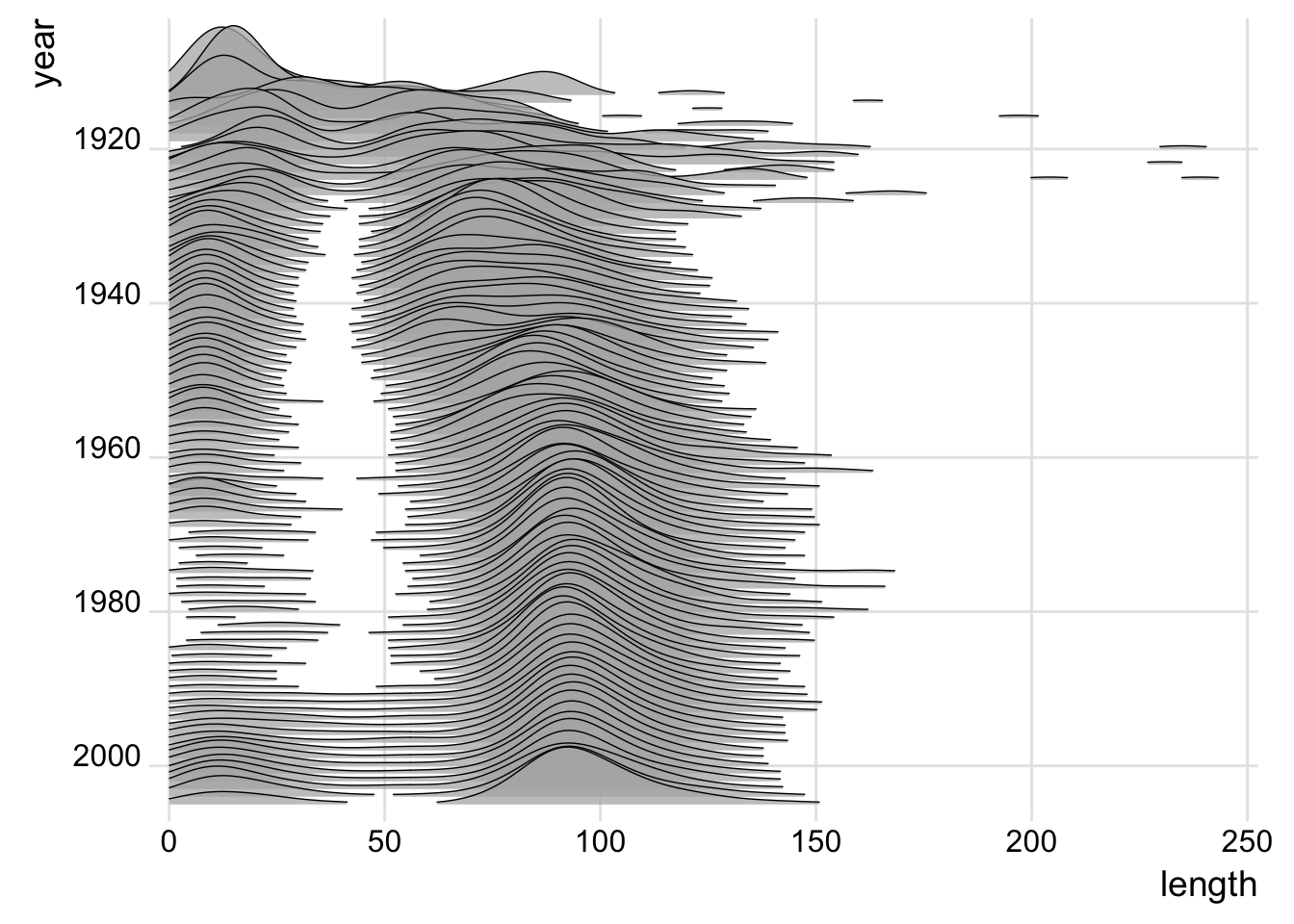
4.10 Ridge plot–An array of density plots

https://cran.r-project.org/web/packages/ggridges/vignettes/gallery.html

library(ggridges)
library(ggplot2movies)

movies %>% filter(year>1912, length<250) %>% 
ggplot(aes(x = length, y = year, group = year)) +
  geom_density_ridges(scale = 10, size = 0.25, rel_min_height = 0.03, alpha=.75) +
  scale_x_continuous(limits=c(0, 250), expand = c(0.01, 0)) +
  scale_y_reverse(breaks=c(2000, 1980, 1960, 1940, 1920, 1900), expand = c(0.01, 0)) +
  theme_ridges()

## Picking joint bandwidth of 6.89